Having a way to summarize the contents of a large text corpus can be very interesting. In this example, I will graphically summarize “On the Origin of Species” by Charles Darwin to demonstrate this technique.
These are the libraries I will be using:
library(dplyr)
library(tidytext)
library(tidyverse)
library(topicmodels)
library(RColorBrewer)
I obtained the text of the 1859 edition from Wikisource. The book has 14 chapters which I saved each in its own text file, labeled “chapter01.txt” to “chapter14.txt”. First, I loaded every chapter of the book and stored it in a data frame, with one row for each chapter and 3 columns: book, chapter and text.
#read a text from path x
read <- function(x) {paste(readLines(x), collapse=" ")}
#read origin of species
origin.num.ch <- 14
origin <- character(origin.num.ch)
chapter <- c(1:origin.num.ch)
for (c in chapter) {
   path = paste0(
      "../darwin/origin/chapter",
      sprintf("%02d", c),".txt")
   origin[c] <- read(path)
}
origin.book <- data.frame(
   c("origin of species"),
   c(1:origin.num.ch),
   unlist(origin),
   stringsAsFactors = FALSE)
colnames(origin.book ) <- c("book", "chapter", "text")
Next, cast the corpus to a document term matrix (dtm), that will be used as input for the topic model:
dtm <- origin.book %>%
   unnest_tokens(input="text", output="word") %>%
   anti_join(stop_words) %>%
   count(chapter, word) %>%
   cast_dtm(document=chapter, term=word, value=n)
Finding the best number of topics
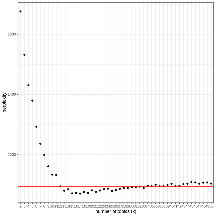
In order to summarize the book, I have to know how many topics it deals with. This is an interesting problem, since for this book as for most texts, there will not be an obvious answer. I used the measure of “perplexity” provided by the “topicmodels” package.
I will try to fit a model, here Latent Dirichlet allocation (LDA) provided by the package “topicmodels”, to a number of topics from 2 to 50.
num.tries = 50
# k=1 doesn't make sense,
# so there are num.tries-1 entries
# in the vector holding perplexities
mod.per = numeric(num.tries-1)
for (i in 2:num.tries) {
   mod <- LDA(
      x=dtm,
      k=i, # k is the number of topics.
      method="Gibbs",
      control=list(alpha=1, seed=10005))
   mod.per[i-1] = perplexity(mod, dtm)
}
# store the result in a data frame for further use
mod.per.df <- data.frame(c(2:num.tries), mod.per)
colnames(mod.per.df) <- c("k", "perplexity")
After having fitted a LDA model for a number of topics between 2 and 50, and calculated its “perplexity” (which takes 20 minutes on my computer), I can now search for the smallest number of topics after which adding new topics does not decrease perplexity.
#set number of topics to
#the first k with lower perplexity than all following k's
min.p <- mod.per.df$perplexity[2]
num.topics <- num.tries
for(i in mod.per.df %>% pull(k)) {
   k.current <- mod.per.df %>%
      filter(k==i) %>%
      pull(perplexity)
   k.following <- max(
      mod.per.df %>%
      filter(k>i) %>%
      pull(perplexity)
   )
   if (k.current < k.following) {
      num.topics <- i
      min.p <- k.current
      break
   }
}
num.topics
In this case, 12 topics seems appropriate. This can be seen on the following plot:
Fit a model, here Latent Dirichlet allocation (LDA) provided by the package “topicmodels”, using the best number of topics as the “k” parameter (here 12).
mod <- LDA(
   x=dtm,
   k=num.topics,
   method="Gibbs",
   control=list(alpha=1, seed=10005)
)
The LDA model return two matrices. The “beta” matrix is the document-term matrix, which describes the words that characterize a topic. Each word is given a value (phi). For each topic, find the words in the document-term matrix where the phi is in the 99.9% quantile, to get a grasp of what each topic is about.
#grab the topic-term matrix
beta <- tidy(mod, matrix="beta")
#add a column with the upper 99.9% quantile of beta for each topic
q <- beta %>%
   select("topic", "beta") %>%
   group_by(topic) %>%
   summarize(quants = quantile(beta, probs = c(0.999))) %>%
   mutate(quants = quants[[1]])
#list the terms with beta in the upper 99.9% quantile for each topic
topics <- beta %>%
   select(c("topic", "term", "beta")) %>%
   group_by(topic) %>%
   arrange(topic, desc(beta)) %>%
   filter(beta > q[topic,]$quants)
I can now print the most characteristic words for each of the 12 topics:
topic.terms = c()
for (t in 1:num.topics) {
   word_frequencies <- tidy(mod, matrix="beta") %>%
      mutate(n = trunc(beta * 10000)) %>%
      filter(topic == t)
topic.string <- paste(topics %>%
   filter(topic == t) %>%
   arrange(term) %>%
   pull(term), collapse=", ")
   print(paste("Topic", t, ":", topic.string))
   topic.terms[t] <- topic.string
}
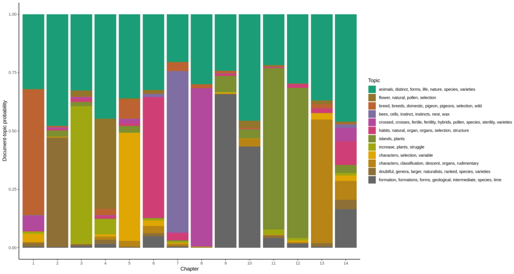
This gives the following topic characterizations:
Topic 1 : animals, distinct, forms, life, nature, species, varieties
Topic 2 : flower, natural, pollen, selection
Topic 3 : breed, breeds, domestic, pigeon, pigeons, selection, wild
Topic 4 : bees, cells, instinct, instincts, nest, wax
Topic 5 : crossed, crosses, fertile, fertility, hybrids, pollen, species, sterility, varieties
Topic 6 : habits, natural, organ, organs, selection, structure
Topic 7 : islands, plants
Topic 8 : increase, plants, struggle
Topic 9 : characters, selection, variable
Topic 10 : characters, classification, descent, organs, rudimentary
Topic 11 : doubtful, genera, larger, naturalists, ranked, species, varieties
Topic 12 : formation, formations, forms, geological, intermediate, species, time”
Now for each chapter, plotting the document-topic probabilities gives the diagram at the top of this post. To do this, I have to use the other matrix returned by the LDA model: the document-topic matrix “gamma”, and plot the chapters on the horizontal axis, the probability that a topic describes a chapter (which is also called “gamma” as is the matrix) is plotted as a color.
# set the size of the diagram
options(repr.plot.width=15, repr.plot.height=8)
# make a palette for the number of topics
mycolors <- colorRampPalette(brewer.pal(8, "Dark2"))(num.topics)
#grab the document-topic matrix
gamma <- tidy(mod, matrix="gamma")
ggplot(gamma,
      # has to be numeric to sort the chapters in the right order
      aes(as.factor(as.numeric(document)),
      gamma,
      # has to be factor to use a discrete color scale
      fill=as.factor(topic))
   ) +
   geom_col() +
   scale_fill_manual(values = mycolors, labels = topic.terms) +
   scale_color_manual(values = mycolors) +
   theme_classic() +
   labs(x="Chapter", y="Document-topic probability", fill="Topic")